LaTeX math in base R graphics • gridmicrotex

Turn on latex_options(device_math = TRUE) and any plot label written with $...$ is typeset as LaTeX. The rest of your plotting code stays the same.

A first plot

library(gridmicrotex)
library(grid)

latex_options(device_math = TRUE)

plot(1:10, (1:10)^2,
     main = r"(Slope $\hat{\beta}_1 = \sum_{i=1}^{n} x_i^2$)",
     xlab = "Cost $5-$10 per unit",
     ylab = r"($\frac{y}{2}$)")
text(3, 80, r"($\int_0^\infty e^{-x^2}\,dx$)", col = "steelblue")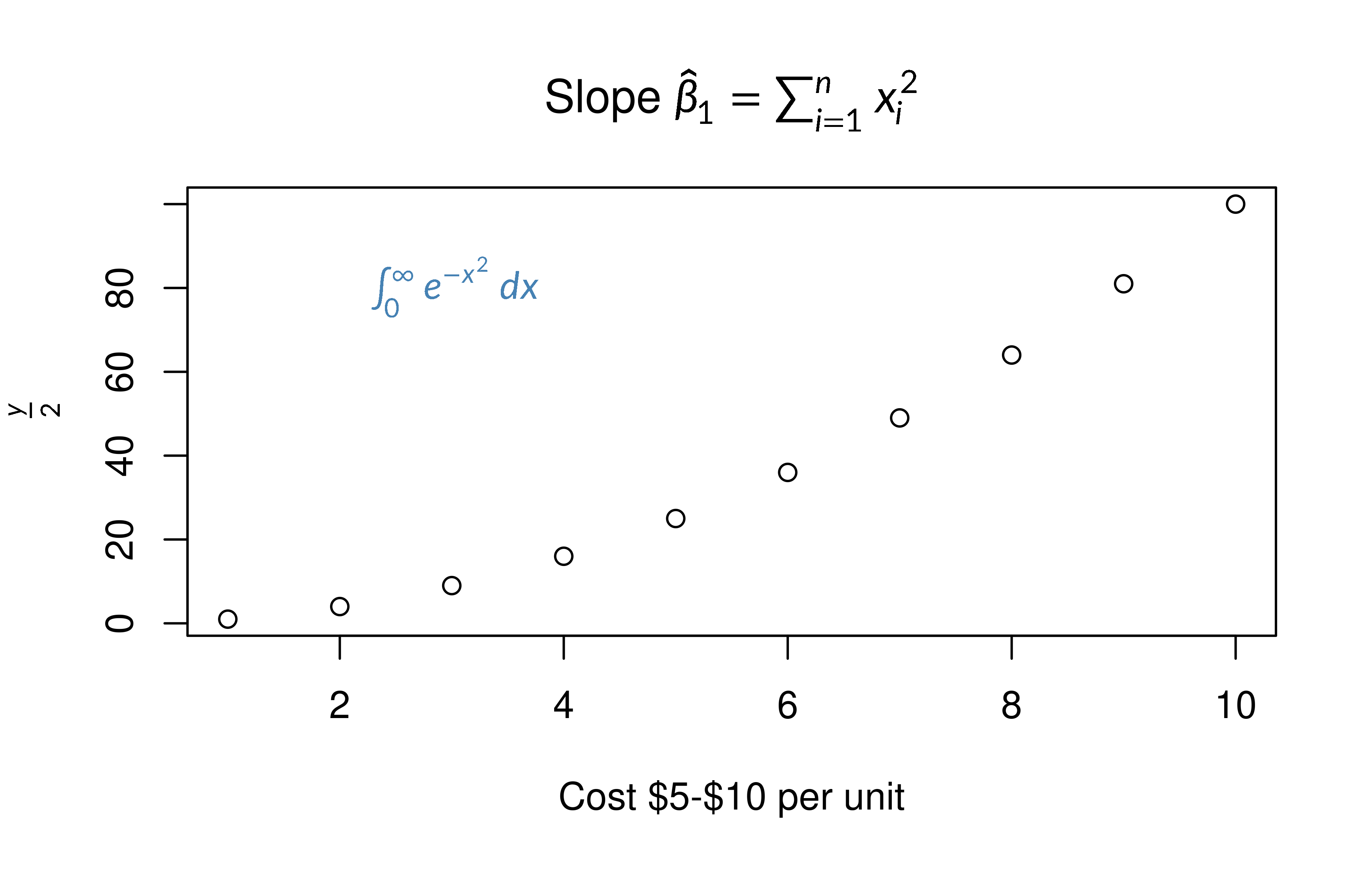

The title, y-axis label and annotation are typeset. The x-axis label has no math in it, so it is drawn as written.

In R Markdown, set the option in the setup chunk. If you turn it off, do so in a later chunk than the plot, or the plot shows the literal $...$ .

More than plotmath

Tables, display-style operators and other LaTeX work in any label. The coefficient table below is drawn by an ordinary text() call:

set.seed(42)
x   <- seq(0, 3, length.out = 60)
y   <- 2 + 1.4 * x^2 + rnorm(60, sd = 1.1)
fit <- lm(y ~ poly(x, 2, raw = TRUE))
cf  <- signif(coef(summary(fit)), 3)

title_eq <- r"($$\hat{y} = \beta_0 + \beta_1 x + \beta_2 x^2$$)"

# Make room for the tall title
h   <- latex_dims(title_eq, gp = gpar(fontsize = par("ps")))$height
top <- ceiling(convertHeight(h, "bigpts", TRUE) /
               (par("cin")[2] * 72 * par("mex"))) + 2

par(mar = c(4.5, 5.5, top, 2))
plot(x, y, pch = 19, col = "grey45", cex = 0.7, ylim = c(0, 22),
     main = title_eq, xlab = r"($x$)",
     ylab = r"($y = f(x) + \varepsilon$)")
lines(x, predict(fit), col = "#B22222", lwd = 2)

# Build the table as a single line of text
tab <- sprintf(paste0(
  r"(\begin{array}{|l|r|r|}\hline)",
  r"(\rowcolor{#E8F0FE}\text{Term} & \hat{\beta} & \text{SE}\\\hline)",
  r"(\beta_0 & %s & %s\\)",
  r"(\beta_1 & %s & %s\\)",
  r"(\beta_2 & %s & %s\\\hline\end{array})"),
  cf[1, 1], cf[1, 2], cf[2, 1], cf[2, 2], cf[3, 1], cf[3, 2])

text(0.05, 18, tab, adj = c(0, 0.5), cex = 0.75)
text(2.95, 1.2, r"($\varepsilon \sim \mathcal{N}(0, \sigma^2)$)",
     adj = c(1, 0), cex = 0.95, col = "#B22222")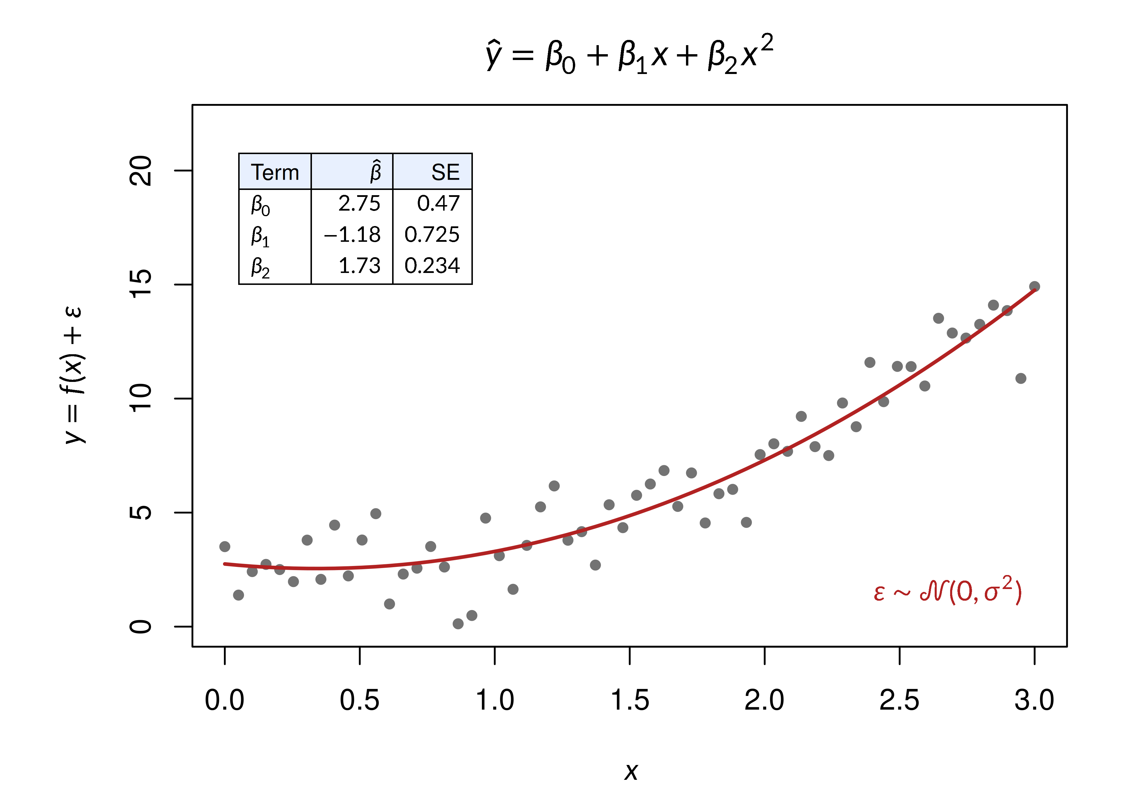

Two tips from this example:

Keep a formula on one line. A label containing a newline is not recognised as math.
Anchor a tall label by its centre (adj = c(0, 0.5)) and leave room around it; see Tall formulas.

Other packages

The option works for any plot drawn on an R graphics device: base plot methods such as plot(lm), hist() and legend(), lattice, grid, and ggplot2 (axis titles, geom_text(), facet strips, legend keys). It does not reach plotly or rgl’s text3d() labels.

For ggplot2, geom_latex() and element_latex() are often the better choice; see vignette("ggplot2-integration").

When is a label treated as math?

A label is typeset only when every $ in it is closed and each $...$ pair holds something that looks like math. Everyday dollar signs are left alone:

Label	Rendered as
`"Revenue ($)"`	text
`"Price is $5 today"`	text
`"Cost $5-$10"`	text
`"Budget $1,000 to $5,000 with $x$ shown"`	text
`"Histogram of df$a_b - df$c_d"`	text
`"$x$"`	math
`"$x^2$"`	math
`"$y = 2x + 1$"`	math
`"Slope $\\hat{\\beta}_1$"`	math
`"\$\\alpha\$"`	math

$$...$$, $...$ and \[...\] also work. Write \$ for a literal dollar sign in a label that also has math.

Tall formulas

Widths are measured correctly, but heights are not: R sizes margins, titles and legend() boxes for one line of text, so a tall formula can overflow them. Measure it with latex_dims() and widen the margin:

h  <- latex_dims(r"($\frac{a}{b}$)", gp = gpar(fontsize = par("ps")))$height
bp <- convertHeight(h, "bigpts", TRUE)

# Lines of margin needed
bp / (par("cin")[2] * 72 * par("mex"))
#> [1] 1.041667

Round that up and add it to the matching side of par(mar = ).

Limitations

The option applies to every plot in the session, including plots from other packages. Labels without math are not changed.
Math is drawn as outlines, so it cannot be selected in a PDF or SVG.
Bold comes from \textbf{}, not from the plot’s font face.
\includegraphics is skipped, and rounded box corners are square.
A label that cannot be read is drawn as plain text, without a warning.
It does not work together with showtext::showtext_auto().
expression() labels are not affected.
corrplot reads a label starting with $ itself; start it with something else.