gridmicrotex provides two ggplot2 extensions for rendering LaTeX math in plots:
-
geom_latex()— a geom layer for placing LaTeX labels at data coordinates. -
element_latex()— a theme element for rendering axis titles, plot titles, and other text elements as LaTeX.
Annotating plots with geom_latex()
geom_latex() works like geom_text() but
interprets the label aesthetic as a LaTeX math string. You
can also map the size (font size in points) and
colour aesthetics as usual. element_latex()
replaces a text theme element so that its label is rendered as LaTeX
math.
df <- data.frame(
  x = 1:3,
  y = 1:3,
  eq = c("$x^2$", "\\frac{a}{b}", "$\\sum_{i=1}^n x_i$"),
  col = c("red", "blue", "green")
)

ggplot(df, aes(x, y,
               label = eq,
               colour = col,
               size = c(14, 18, 14))) +
  geom_latex() +
  scale_colour_identity() +
  scale_size_identity() +
  labs(
    x = "$\\beta_1 \\cdot x + \\beta_0$",
    y = "$\\mathrm{mpg}$"
  ) +
  theme(
    axis.title.x = element_latex(fontsize = 14),
    axis.title.y = element_latex(fontsize = 14)
  )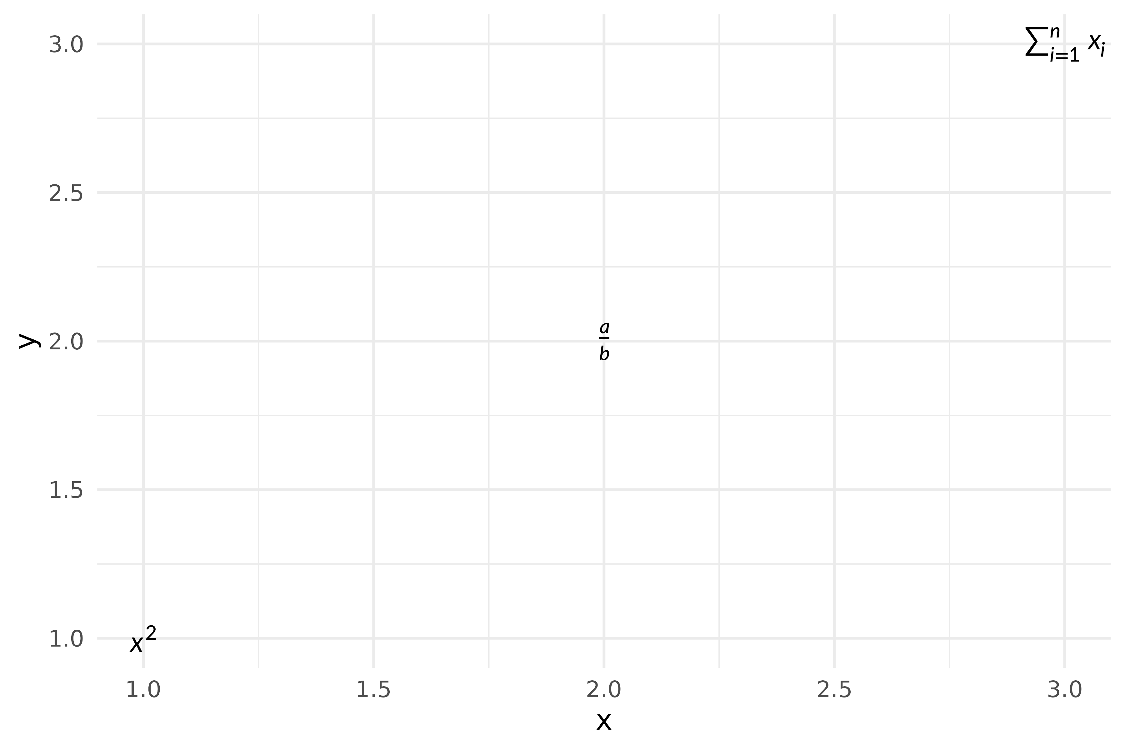
Dollar-sign delimiters ($...$) are stripped
automatically, so both "\\frac{a}{b}" and
"$\\frac{a}{b}$" produce the same output.
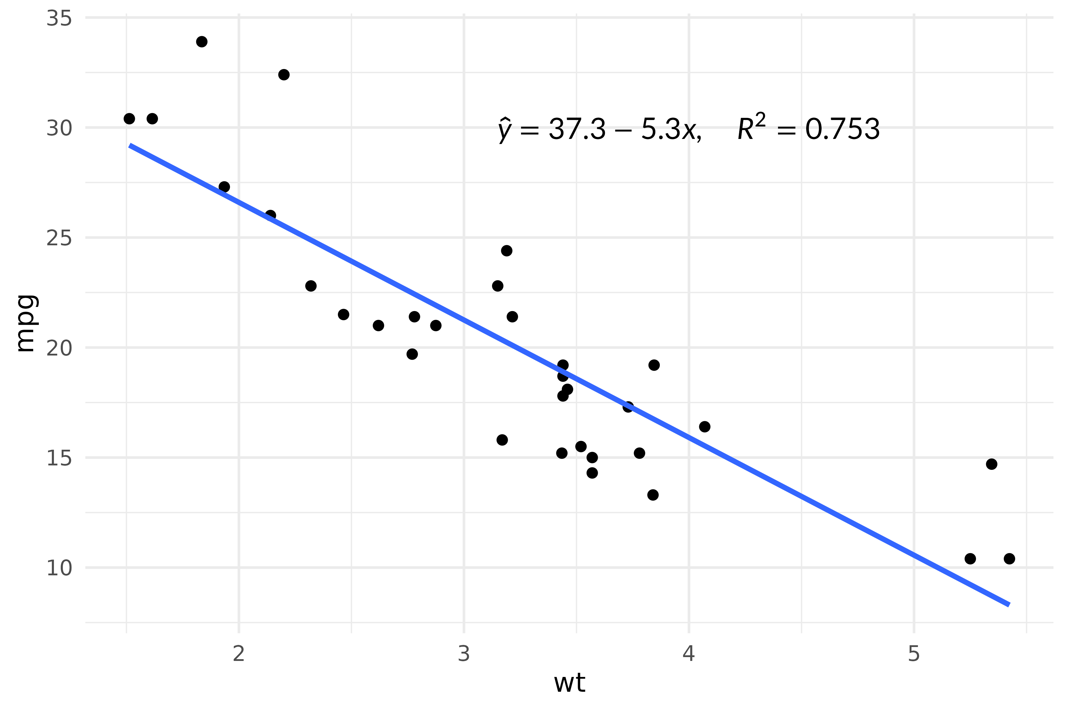
Adding equation annotations to a scatter plot
A common use case is annotating a regression fit with the model
equation. Use annotate("latex", ...) for single annotations
— it delegates to GeomLatex internally but avoids creating
a data frame and automatically hides the legend.
fit <- lm(mpg ~ wt, data = mtcars)
b0 <- round(coef(fit)[1], 1)
b1 <- round(coef(fit)[2], 1)
r2 <- round(summary(fit)$r.squared, 3)

eq_label <- sprintf("$\\hat{y} = %s %s x, \\quad R^2 = %s$",
                     b0, b1, r2)

ggplot(mtcars, aes(wt, mpg)) +
  geom_point() +
  geom_smooth(method = "lm", se = FALSE) +
  annotate("latex", x = 4, y = 30, label = eq_label, size = 12) +
  theme_minimal()
#> `geom_smooth()` using formula = 'y ~ x'