A ggplot2 geom for LaTeX math labels — geom

Like ggplot2::geom_text(), with labels written in LaTeX. The $ signs are optional. annotate("latex", ...) adds a single label.

Usage

geom_latex(
  mapping = NULL,
  data = NULL,
  stat = "identity",
  position = "identity",
  ...,
  fontsize = 11,
  math_font = "",
  lineheight = 1.2,
  max_width = 0,
  input_mode = c("mixed", "math", "document"),
  render_mode = c("typeface", "path"),
  na.rm = FALSE,
  show.legend = NA,
  inherit.aes = TRUE
)

Arguments

mapping

Set of aesthetic mappings created by aes(). If specified and inherit.aes = TRUE (the default), it is combined with the default mapping at the top level of the plot. You must supply mapping if there is no plot mapping.

data

The data to be displayed in this layer. There are three options:

If NULL, the default, the data is inherited from the plot data as specified in the call to ggplot().

A data.frame, or other object, will override the plot data. All objects will be fortified to produce a data frame. See fortify() for which variables will be created.

A function will be called with a single argument, the plot data. The return value must be a data.frame, and will be used as the layer data. A function can be created from a formula (e.g. ~ head(.x, 10)).

stat

The statistical transformation to use on the data for this layer. When using a geom_*() function to construct a layer, the stat argument can be used to override the default coupling between geoms and stats. The stat argument accepts the following:

A Stat ggproto subclass, for example StatCount.
A string naming the stat. To give the stat as a string, strip the function name of the stat_ prefix. For example, to use stat_count(), give the stat as "count".
For more information and other ways to specify the stat, see the layer stat documentation.

position

A position adjustment to use on the data for this layer. This can be used in various ways, including to prevent overplotting and improving the display. The position argument accepts the following:

The result of calling a position function, such as position_jitter(). This method allows for passing extra arguments to the position.
A string naming the position adjustment. To give the position as a string, strip the function name of the position_ prefix. For example, to use position_jitter(), give the position as "jitter".
For more information and other ways to specify the position, see the layer position documentation.

...

Passed to ggplot2::layer().

fontsize

Font size in points, unless size is mapped.

math_font

Math font, such as "stix".

lineheight

Line spacing (default 1.2).

max_width

Width in big points at which lines wrap. 0, the default, does not wrap.

input_mode

How tex is read:

"mixed" (default): text, with math between $...$ or $...$. A newline starts a new line.
"math": everything is math; write text in \text{}.
"document": a LaTeX document body, with paragraphs, numbered headings and displayed equations. Use it with max_width.

render_mode

"typeface" (default) draws glyphs as text, which can be selected in PDF and SVG output. It needs a device such as ragg, svglite or grDevices::cairo_pdf(), and falls back to "path" on others, such as pdf(). "path" draws glyphs as outlines, which works on every device.

na.rm

If FALSE (default), missing values are removed with a warning; if TRUE, silently.

show.legend

logical. Should this layer be included in the legends? NA, the default, includes if any aesthetics are mapped. FALSE never includes, and TRUE always includes. It can also be a named logical vector to finely select the aesthetics to display. To include legend keys for all levels, even when no data exists, use TRUE. If NA, all levels are shown in legend, but unobserved levels are omitted.

inherit.aes

If FALSE, overrides the default aesthetics, rather than combining with them. This is most useful for helper functions that define both data and aesthetics and shouldn't inherit behaviour from the default plot specification, e.g. annotation_borders().

Value

A ggplot2 layer.

Aesthetics

geom_latex() understands the following aesthetics (required aesthetics are in bold):

x
y
label: LaTeX string
size: font size in points (default: 11)
colour: text colour (default: "black")
angle: rotation angle in degrees (default: 0)
hjust: horizontal justification, 0-1 (default: 0.5)
vjust: vertical justification, 0-1 (default: 0.5)
alpha: transparency (default: 1)

Examples

# \donttest{
if (requireNamespace("ggplot2", quietly = TRUE)) {
  library(ggplot2)
  df <- data.frame(
    x = 1:3, y = 1:3,
    eq = c("$x^2$", "$\\frac{a}{b}$", "$\\sum_{i=1}^n x_i$")
  )
  ggplot(df, aes(x, y, label = eq)) + geom_latex()

  # Use annotate() for single annotations (no legend, no data frame needed)
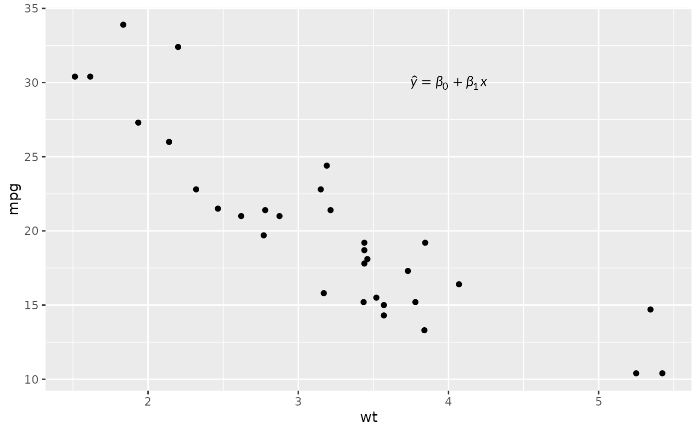
  ggplot(mtcars, aes(wt, mpg)) + geom_point() +
    annotate("latex", x = 4, y = 30,
             label = r"($\hat{y} = \beta_0 + \beta_1 x$)")
}

# }