Introduction to gridmicrotex • gridmicrotex

What is gridmicrotex?

gridmicrotex renders LaTeX math equations as native R grid graphics objects (grobs). It uses the MicroTeX C++ library as its layout engine — MicroTeX parses LaTeX, builds the TeX box model, and computes exact glyph coordinates. The package intercepts this layout data and maps it to native grid primitives (pathGrob, segmentsGrob, rectGrob, textGrob), producing a gTree that works on any R graphics device at any resolution.

Key features:

No external LaTeX installation required — MicroTeX is fully embedded
Resolution-independent vector output on all R devices (PNG, PDF, SVG, …)
Full math support: fractions, roots, integrals, matrices, Greek letters, accents, delimiters, and more
Multiple math fonts (Latin Modern Math, STIX Two Math, Lete Sans Math, TeX Gyre DejaVu Math)
Color support via \textcolor{}
ggplot2 integration with geom_latex() and element_latex()
CJK and multilingual text in \text{} blocks

Basic usage

The core function is latex_grob(), which returns a grid grob:

g <- latex_grob("\\frac{-b \\pm \\sqrt{b^2 - 4ac}}{2a}", gp = grid::gpar(fontsize = 24))
grid::grid.newpage()
grid::grid.draw(g)

For quick rendering, use grid.latex():

grid::grid.newpage()
grid.latex("\\sum_{i=1}^{n} x_i^2", gp = grid::gpar(fontsize = 28))

Positioning and justification

Control placement with x, y, hjust, and vjust:

grid::grid.newpage()
grid.latex("E = mc^2", x = 0.2, y = 0.7, hjust = 0, gp = grid::gpar(fontsize = 24))
grid.latex("F = ma", x = 0.2, y = 0.3, hjust = 0, gp = grid::gpar(fontsize = 24))

Colors

Set the formula color via gp, or use \textcolor{} within the LaTeX:

grid::grid.newpage()
grid.latex(
  "\\textcolor{red}{\\alpha} + \\textcolor{blue}{\\beta} = \\gamma",
  gp = grid::gpar(fontsize = 28)
)

Math fonts

The package bundles Lete Sans Math (default — pairs with R’s default sans text), Latin Modern Math, STIX Two Math, and TeX Gyre DejaVu Math. For most users, the easiest workflow is:

List available math fonts with available_math_fonts()
Select one with latex_options(math_font = ...)
Render formulas normally (no OTF/CLM paths needed)

available_math_fonts()
#> [1] "LatinModernMath-Regular"   "Lete Sans Math"           
#> [3] "STIX Two Math"             "TeXGyreDejaVuMath-Regular"

latex_options(math_font = "stix")
grid::grid.newpage()
grid.latex("\\int_0^1 f(x)\\,dx", gp = grid::gpar(fontsize = 24))


# Switch back to the default (Lete Sans Math)
latex_options(math_font = "lete")

You can still override the font per call via math_font:

grid::grid.newpage()
grid::pushViewport(grid::viewport(layout = grid::grid.layout(2, 1)))
grid::pushViewport(grid::viewport(layout.pos.row = 1))
grid.latex("\\int_0^1 f(x)\\,dx", gp = grid::gpar(fontsize = 24))
grid::upViewport()
grid::pushViewport(grid::viewport(layout.pos.row = 2))
grid.latex("\\int_0^1 f(x)\\,dx", gp = grid::gpar(fontsize = 24), math_font = "stix")
grid::upViewport(2)

Use available_math_fonts() to list loaded fonts and check_fonts() for a diagnostic report.

Advanced: loading custom fonts

Use load_font() only when you need a custom font that is not already bundled/loaded. In the current engine, custom loading still needs a matching CLM metrics file (auto-discovered when possible):

load_font("path/to/MyFont.otf")

You can generate your font CLM using the bundled Python script. See help for load_font() for instructions.

Render modes

gridmicrotex supports two rendering modes for math glyphs:

"typeface" (default): Renders glyphs as native text using the math font’s typeface. This produces selectable, searchable, and accessible text in PDF and SVG output. Requires the math font (e.g., Lete Sans Math) to be installed on the system, and a device that supports font embedding (e.g., ragg::agg_png(), svglite::svglite(), grDevices::cairo_pdf()). On devices that do not support typeface rendering (e.g., the base pdf() device), the package automatically falls back to path mode with a warning.
"path": Renders each glyph as a filled vector path. This works on all R graphics devices and produces pixel-perfect output. However, text in PDF/SVG output is not selectable or searchable.

# Default typeface mode (selectable text in PDF/SVG)
grid.latex("E = mc^2", gp = grid::gpar(fontsize = 24))

# Explicit path mode (works everywhere, but text is not selectable)
grid.latex("E = mc^2", gp = grid::gpar(fontsize = 24), render_mode = "path")

Important: Do not use showtext::showtext_auto() with typeface mode. The showtext package globally intercepts all text rendering and converts it to vector paths. This silently defeats typeface mode, causing all math glyphs to appear as paths instead of native text — even on devices like svglite and ragg that fully support font embedding. If you need showtext for other parts of your plot, disable it before drawing LaTeX formulas:
showtext::showtext_auto(FALSE)
grid.latex("E = mc^2", gp = grid::gpar(fontsize = 24))  # typeface mode works correctly

Querying dimensions

latex_dims() returns the bounding box of an expression:

dims <- latex_dims("\\frac{a}{b}", gp = grid::gpar(fontsize = 20))
dims
#> $width
#> [1] 7bigpts
#> 
#> $height
#> [1] 25bigpts
#> 
#> $depth
#> [1] 9bigpts
#> 
#> $baseline
#> [1] 9.35305953025818bigpts
#> 
#> $is_split
#> [1] FALSE

This is useful for layout calculations and ensuring labels fit.

Text rendering and CJK support

Text inside \text{} and \mbox{} is rendered using R’s standard text-rendering system. This means gp$fontfamily controls the font for all text content — Latin letters, CJK characters, Cyrillic, and any other script your R graphics device supports:

grid::grid.newpage()
grid.latex("x^2 + \\text{你好}", gp = grid::gpar(fontsize = 24, fontfamily = "sans"))

Any font available to R works: base families like "sans", "serif", "mono", or fonts registered via showtext / systemfonts.

Font pairing

The bundled math fonts have different styles. For a consistent look, pair them with a matching fontfamily:

Math font	Style	Suggested `fontfamily`
Lete Sans Math (`"lete"`, default)	Sans-serif	`"sans"`
TeX Gyre DejaVu Math (`"dejavu"`)	Sans-serif	`"sans"`
Latin Modern Math (`"lm"`)	Serif	`"serif"`
STIX Two Math (`"stix"`)	Serif	`"serif"`

grid::grid.newpage()
grid.latex(
  "\\text{Theorem: } \\forall x \\in \\mathbb{R},\\; x^2 \\geq 0",
  math_font = "dejavu",
  gp = grid::gpar(fontfamily = "sans", fontsize = 12)
)

Supported LaTeX

gridmicrotex uses the MicroTeX engine, which is a math formula renderer, not a full document typesetter. It covers the vast majority of math notation you would use in plots and figures, but does not attempt to replace a full LaTeX installation.

Complicated examples

grid::grid.newpage()
grid.latex(paste0(
      "\\begin{array}{l}",
      "  \\forall\\varepsilon\\in\\mathbb{R}_+^*\\ \\exists\\eta>0",
      "\\ |x-x_0|\\leq\\eta\\Longrightarrow|f(x)-f(x_0)|\\leq\\varepsilon\\\\",
      "  \\det",
      "  \\begin{bmatrix}",
      "      a_{11}&a_{12}&\\cdots&a_{1n}\\\\",
      "      a_{21}&\\ddots&&\\vdots\\\\",
      "      \\vdots&&\\ddots&\\vdots\\\\",
      "      a_{n1}&\\cdots&\\cdots&a_{nn}",
      "  \\end{bmatrix}",
      "  \\overset{\\mathrm{def}}{=}\\sum_{\\sigma\\in\\mathfrak{S}_n}",
      "\\varepsilon(\\sigma)\\prod_{k=1}^n a_{k\\sigma(k)}\\\\",
      "  \\int_0^\\infty{x^{2n} e^{-a x^2}\\,dx} = \\frac{2n-1}{2a}",
      " \\int_0^\\infty{x^{2(n-1)} e^{-a x^2}\\,dx}",
      " = \\frac{(2n-1)!!}{2^{n+1}} \\sqrt{\\frac{\\pi}{a^{2n+1}}}\\\\",
      "\\end{array}"
), gp = grid::gpar(fontsize = 16))

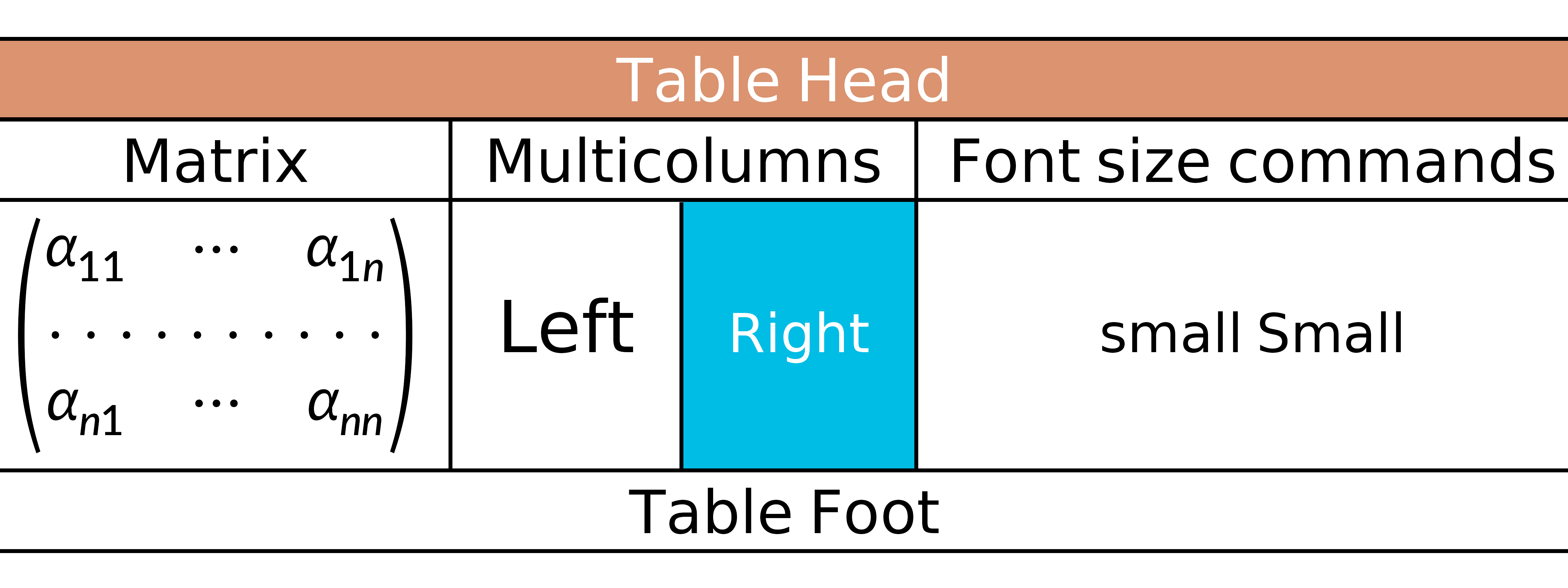
grid::grid.newpage()

grid.latex(
  "
  \\newcolumntype{s}{>{\\color{#1234B6}}c}
\\begin{array}{|c|c|c|s|}
  \\hline
  \\rowcolor{Tan}\\multicolumn{4}{|c|}{\\textcolor{white}{\\bold{\\text{Table Head}}}}\\\\
  \\hline
  \\text{Matrix}&\\multicolumn{2}{|c|}{\\text{Multicolumns}}&\\text{Font size commands}\\\\
  \\hline
  \\begin{pmatrix}
      \\alpha_{11}&\\cdots&\\alpha_{1n}\\\\
      \\hdotsfor{3}\\\\
      \\alpha_{n1}&\\cdots&\\alpha_{nn}
  \\end{pmatrix}
  &\\large \\text{Left}&\\cellcolor{#00bde5}\\small \\textcolor{white}{\\text{\\bold{Right}}}
  &\\small \\text{small Small}\\\\
  \\hline
  \\multicolumn{4}{|c|}{\\text{Table Foot}}\\\\
  \\hline
\\end{array}
  ",
  gp = grid::gpar(fontsize = 22)
)

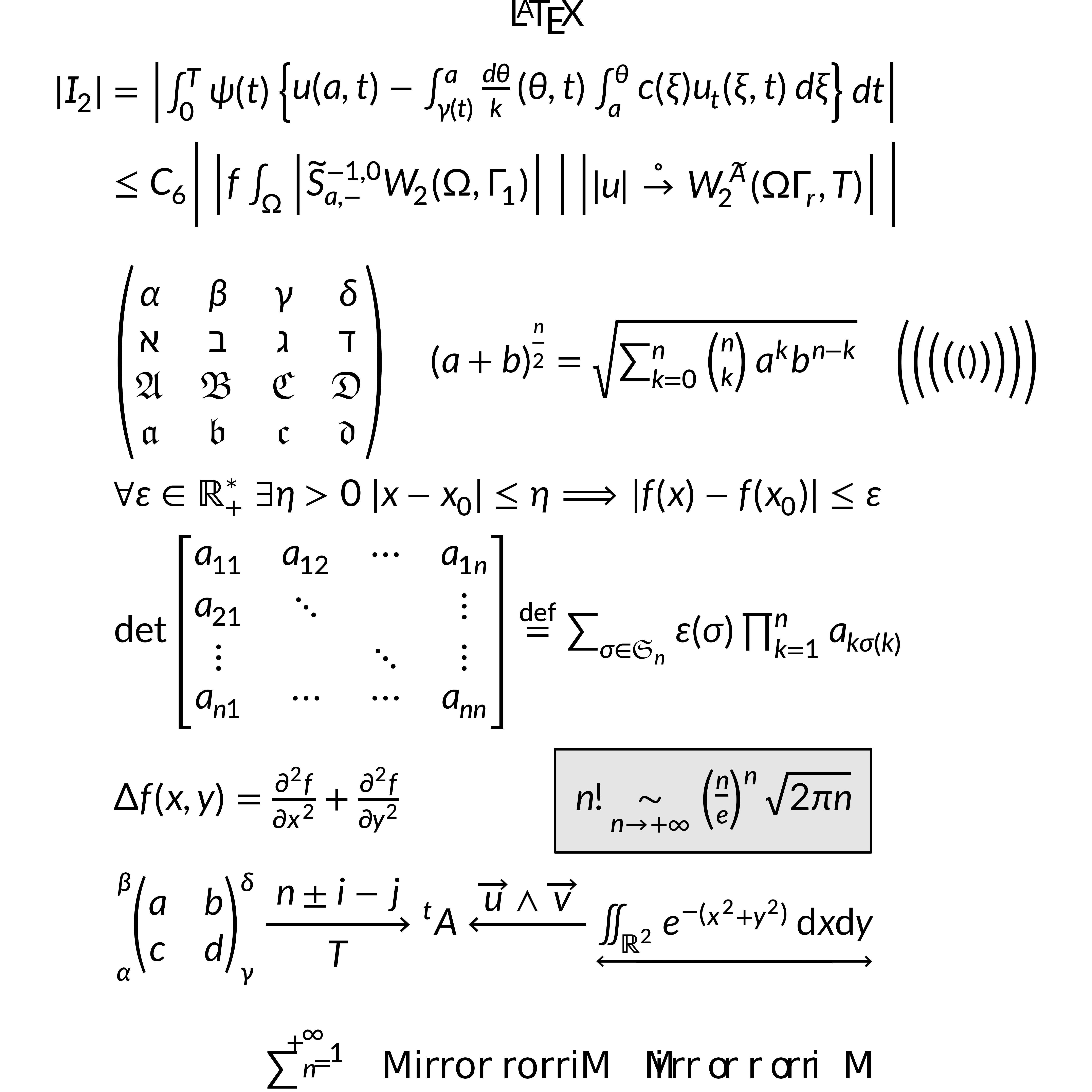
grid::grid.newpage()
grid.latex(
  "\\definecolor{gris}{gray}{0.9}
\\definecolor{noir}{rgb}{0,0,0}
\\definecolor{bleu}{rgb}{0,0,1}
\\fatalIfCmdConflict{false}
\\newcommand{\\pa}{\\left|}
\\begin{array}{c}
  \\LaTeX\\\\
  \\begin{split}
      |I_2| &= \\pa\\int_0^T\\psi(t)\\left\\{ u(a,t)-\\int_{\\gamma(t)}^a \\frac{d\\theta}{k} (\\theta,t) \\int_a^\\theta c(\\xi)
          u_t (\\xi,t)\\,d\\xi\\right\\}dt\\right|\\\\
      &\\le C_6 \\Bigg|\\pa f \\int_\\Omega \\pa\\widetilde{S}^{-1,0}_{a,-}
          W_2(\\Omega, \\Gamma_1)\\right|\\ \\right|\\left| |u|\\overset{\\circ}{\\to} W_2^{\\widetilde{A}}(\\Omega\\Gamma_r,T)\\right|\\Bigg|\\\\
      &\\\\
      &\\begin{pmatrix}
          \\alpha&\\beta&\\gamma&\\delta\\\\
          \\aleph&\\beth&\\gimel&\\daleth\\\\
          \\mathfrak{A}&\\mathfrak{B}&\\mathfrak{C}&\\mathfrak{D}\\\\
          \\boldsymbol{\\mathfrak{a}}&\\boldsymbol{\\mathfrak{b}}&\\boldsymbol{\\mathfrak{c}}&\\boldsymbol{\\mathfrak{d}}
      \\end{pmatrix}
      \\quad{(a+b)}^{\\frac{n}{2}}=\\sqrt{\\sum_{k=0}^n\\tbinom{n}{k}a^kb^{n-k}}\\quad
          \\Biggl(\\biggl(\\Bigl(\\bigl(()\\bigr)\\Bigr)\\biggr)\\Biggr)\\\\
      &\\forall\\varepsilon\\in\\mathbb{R}_+^*\\ \\exists\\eta>0\\ |x-x_0|\\leq\\eta\\Longrightarrow|f(x)-f(x_0)|\\leq\\varepsilon\\\\
      &\\det
      \\begin{bmatrix}
          a_{11}&a_{12}&\\cdots&a_{1n}\\\\
          a_{21}&\\ddots&&\\vdots\\\\
          \\vdots&&\\ddots&\\vdots\\\\
          a_{n1}&\\cdots&\\cdots&a_{nn}
      \\end{bmatrix}
      \\overset{\\mathrm{def}}{=}\\sum_{\\sigma\\in\\mathfrak{S}_n}\\varepsilon(\\sigma)\\prod_{k=1}^n a_{k\\sigma(k)}\\\\
      &\\Delta f(x,y)=\\frac{\\partial^2f}{\\partial x^2}+\\frac{\\partial^2f}{\\partial y^2}\\qquad\\qquad \\fcolorbox{noir}{gris}
          {n!\\underset{n\\rightarrow+\\infty}{\\sim} {\\left(\\frac{n}{e}\\right)}^n\\sqrt{2\\pi n}}\\\\
      &\\sideset{_\\alpha^\\beta}{_\\gamma^\\delta}{
      \\begin{pmatrix}
          a&b\\\\
          c&d
      \\end{pmatrix}}
      \\xrightarrow[T]{n\\pm i-j}\\sideset{^t}{}A\\xleftarrow{\\overrightarrow{u}\\wedge\\overrightarrow{v}}
          \\underleftrightarrow{\\iint_{\\mathds{R}^2}e^{-\\left(x^2+y^2\\right)}\\,\\mathrm{d}x\\mathrm{d}y}
  \\end{split}\\\\
  \\rotatebox{30}{\\sum_{n=1}^{+\\infty}}\\quad\\mbox{Mirror rorriM}\\reflectbox{\\mbox{Mirror rorriM}}
\\end{array}",
  gp = grid::gpar(fontsize = 22)
)

What is not supported

MicroTeX is a math formula renderer, not a full LaTeX engine. The following are outside its scope:

Document structure: \section, \begin{document}, page layout, headers/footers, \tableofcontents
Package loading: \usepackage{} — all supported commands are built in
Paragraph text: line breaking, hyphenation, justified paragraphs
TikZ / PGF drawing commands
Images: \includegraphics
Cross-references: \label, \ref, \cite, bibliographies
Theorem environments: \begin{theorem}, \begin{proof}
Lists: itemize, enumerate, description
Some amsmath commands: \substack, \tag, equation numbering

For most statistical graphics use cases — axis labels, annotations, legends, and in-plot formulas — the supported feature set is more than sufficient.

Project-wide defaults

latex_options() sets defaults for math_font and render_mode, used by latex_grob(), grid.latex(), latex_dims(), and latex_tree() whenever the corresponding argument is not supplied at the call site. Size is controlled at the grob level via gp$fontsize / gp$lineheight (see Basic usage).

latex_options(math_font = "stix", render_mode = "typeface")

# Later calls pick these up automatically
grid.latex("\\sum_{i=1}^{n} i^{2}", gp = grid::gpar(fontsize = 14))

# Query current settings
latex_options()

# Reset to built-in defaults
reset_latex_options()

Explicit arguments always win. Setting math_font via latex_options() also updates the MicroTeX engine default, so you don’t also need a separate font-setup call.

User-defined macros

define_macro() registers zero-argument shorthands that are expanded by text substitution before the expression reaches MicroTeX. Handy for recurring notation:

define_macro("RR", "\\mathbb{R}")
define_macro("eps", "\\varepsilon")

grid::grid.newpage()
grid.latex("\\forall \\eps > 0, \\eps \\in \\RR", gp = grid::gpar(fontsize = 24))


clear_macros()

Macro names must be ASCII letters. Expansion iterates to a fixed point, so macros can reference other macros. Use list_macros() to see currently registered ones, and clear_macros() (with no arguments) to drop them all.

Layout caching

Parsed layouts are memoised by (tex, fontsize, math_font, render_mode, ...). Re-drawing the same formula — for example, the same axis label across many plots — reuses the cached layout:

latex_cache_info()       # size / max_size / hits / misses
latex_cache_limit(1024)  # raise or lower the LRU capacity
latex_cache_clear()      # wipe the cache (e.g. after re-loading fonts)

Set the limit to 0 to disable caching entirely.

Introspecting a formula

latex_tree() returns the raw draw-record table plus bbox metadata, useful for debugging alignment, counting glyphs, or building custom grobs on top of the layout:

tr <- latex_tree("\\frac{a}{b}")
tr
#> <latex_tree>
#>   tex:         \frac{a}{b}
#>   render_mode: typeface
#>   bbox:        width=7.00  height=25.00  depth=9.00  baseline=0.63 (bigpts)
#>   records:     3
#>     glyph      2
#>     line       1
head(tr$records, 3)
#>    type     x      y glyph font_size   color    x2     y2 width height rx ry
#> 1 glyph 0.175  7.224  2701        14 #000000    NA     NA    NA     NA NA NA
#> 2  line 0.000 10.624    NA        NA #000000 7.392 10.624    NA     NA NA NA
#> 3 glyph 0.000 25.824  2702        14 #000000    NA     NA    NA     NA NA NA
#>    lwd text font_style path codepoint
#> 1   NA <NA>         NA NULL        NA
#> 2 1.32 <NA>         NA NULL        NA
#> 3   NA <NA>         NA NULL        NA
#>                                                             font_file
#> 1 /home/runner/work/_temp/Library/gridmicrotex/fonts/LeteSansMath.otf
#> 2                                                                <NA>
#> 3 /home/runner/work/_temp/Library/gridmicrotex/fonts/LeteSansMath.otf

Debug overlay

Pass debug = TRUE to latex_grob() / grid.latex() to overlay diagnostics on the rendered formula — the full bounding box (dashed gray), the baseline (solid red), and a dot at each draw record’s origin. Useful for checking vertical alignment between a formula and surrounding grobs:

grid::grid.newpage()
grid.latex("x^{2} + y_{i}", gp = grid::gpar(fontsize = 30), debug = TRUE)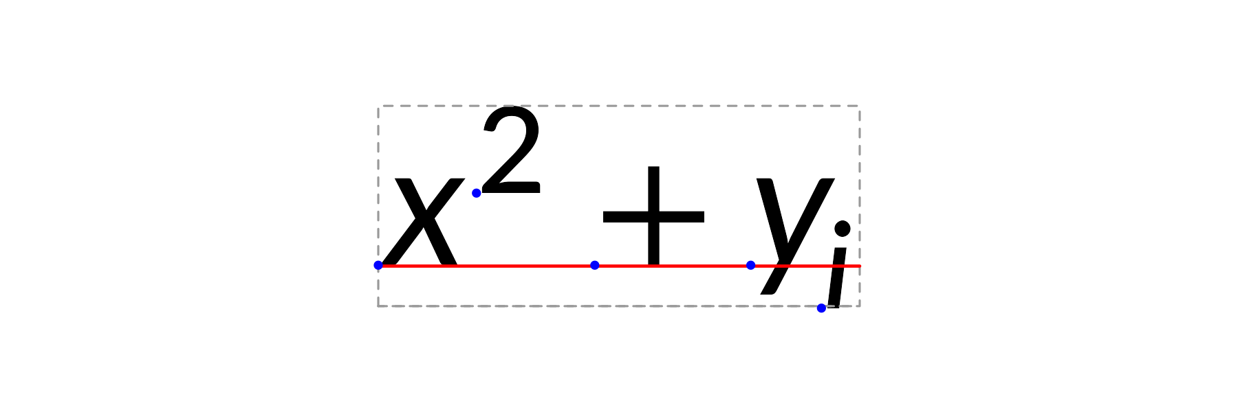

Comparison with alternatives

Approach	LaTeX required?	Device independent?	Vector?	Math coverage
`tikzDevice`	Yes	No	Yes	Full
`xdvir`	Yes	No	Yes	Full
`latexpdf`	Yes	No	Yes	Full (tables)
`latex2exp`	No	Yes	Yes	Limited
`plotmath`	No	Yes	Yes	Limited
gridmicrotex	No	Yes	Yes	Broad

Graphics backend

The default graphics device on Windows (windows()) and macOS (quartz()) may not find the bundled math fonts, producing warnings like:

font family not found in Windows font database

To avoid this, switch to a modern graphics backend that uses systemfonts for font resolution:

# For knitr / R Markdown --- add to your setup chunk:
knitr::opts_chunk$set(dev = "ragg_png")

# For interactive use:
options(device = function(...) ragg::agg_png(tempfile(fileext = ".png"), ...))

Recommended backends:

Backend	Format	Package
`ragg::agg_png()`	PNG	ragg
`svglite::svglite()`	SVG	svglite
`grDevices::cairo_pdf()`	PDF	Base R (Cairo build)

Alternatively, use render_mode = "path" to bypass font lookup entirely — glyphs are drawn as vector paths, which works on all devices but produces non-selectable text in PDF/SVG.