Scale point sizes by weights

Read the sizes given to forest as study weights and turn them into point sizes. The square root of the weights is taken first, so that the area of each point is proportional to its weight, before mapping onto range.

Usage

scale_sizes(plot, method = c("range", "proportional"), range = c(0.2, 0.8))

Arguments

plot

A forest plot object, see forest.

method

"range" (default) puts the smallest weight on range[1] and the largest on range[2], as metafor::forest.rma does with its plim. "proportional" keeps the areas proportional to the weights and only clamps the smallest points up, as meta::forest.meta does.

range

Numeric vector of length 2 giving the smallest and largest point size, as a multiple of one line of text.

Value

A forest plot object.

Details

Weights are scaled jointly across all groups and CI columns so that the areas stay comparable between them; scale by hand if per-column control is wanted. Rows flagged by is_summary are held out of the scaling and drawn at range[2], since a pooled total is not comparable with a study weight. This follows meta, whose pooled rows carry no study weight and end up the size of the largest study square, and metafor, which sizes its summary polygon from efac rather than from the weights.

Each call sets both the method and the range, and method = NULL turns the scaling off, so that sizes are used as they are.

See also

forest

Examples

library(grid)
# Read provided sample example data
dt <- read.csv(system.file("extdata", "example_data.csv", package = "forestploter"))
dt <- dt[1:6, ]

# Add a blank column for the forest plot to display CI
dt$` ` <- paste(rep(" ", 20), collapse = " ")

# The weight of each study, here the inverse of the width of the CI
weights <- 1/(dt$hi - dt$low)

p <- forest(dt[, c("Subgroup", " ")],
            est = dt$est,
            lower = dt$low,
            upper = dt$hi,
            sizes = weights,        # weights, not sizes
            ci_column = 2,
            ref_line = 1)

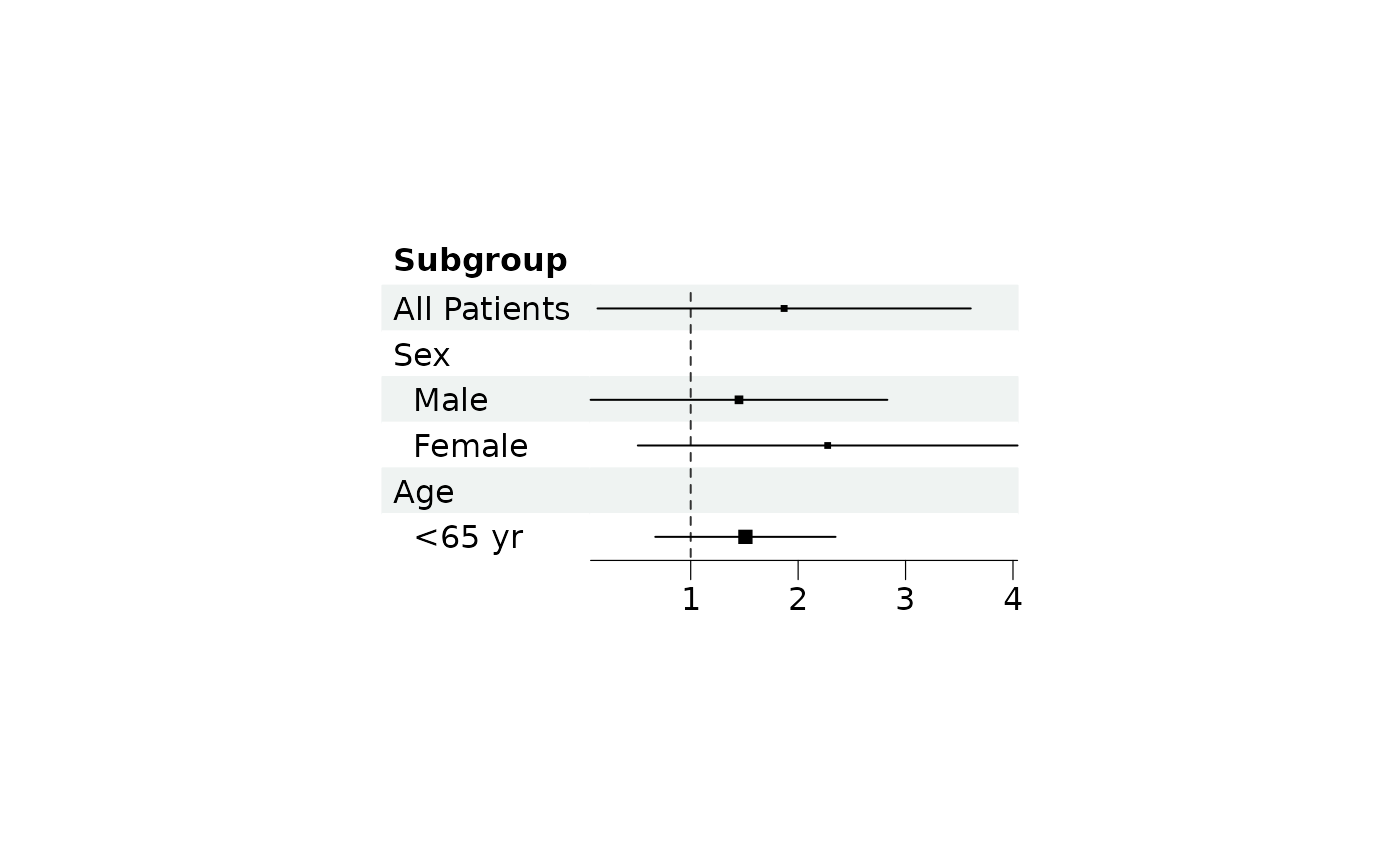
# The area of each point is proportional to its weight
plot(scale_sizes(p, method = "range", range = c(0.2, 0.8)))


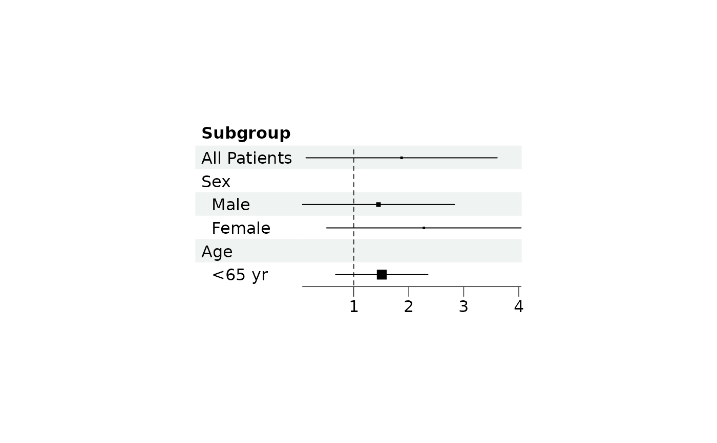# `NULL` turns the scaling off, the values of `sizes` are then used as they are
plot(scale_sizes(p, method = NULL))